Bringing Carleman Estimates to the Grid

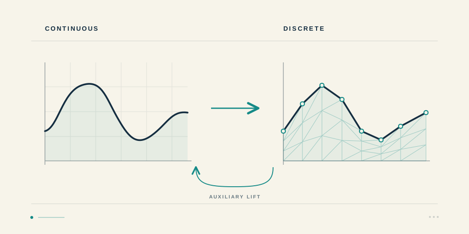
Suppose a continuous equation already has a Carleman estimate. Can we carry that estimate over to a numerical scheme?

For numerical control, this matters beyond convergence of the state equation. A convergent approximation of the heat equation does not automatically produce controls whose cost stays bounded as the grid is refined. Nor does it guarantee a vanishing terminal error.

Our paper develops a transfer principle based on weighted numerical error estimates.¹ Before adding time discretization, a Poisson problem from the introduction makes the central construction visible.

Convergence misses the highest frequencies

On \((0,1)\) with homogeneous Dirichlet conditions, the sine modes have continuous and centered-difference eigenvalues

For a fixed \(j\), the relative error tends to zero as \(h\to0\). But the highest discrete mode behaves differently:

Consistency on fixed smooth functions does not give a small perturbation uniformly over the discrete space. Mesh-scale oscillations remain.

A Carleman estimate also carries a large parameter \(s\). Increasing it makes the exponential weight vary more sharply and tightens the error-absorption condition. The perturbation argument discussed in the paper requires a quantity of the form \(Cs\|\varepsilon\|_\infty^2\) to be small. A relative error that stays away from zero cannot support a growing range of \(s\).

Simply interpolating the discrete state does not remove the difficulty. A piecewise-linear finite-element function generally has only \(H^1\) regularity. Taking its second derivatives element by element misses the jumps in its gradient across interfaces. The continuous residual cannot simply be replaced by the discrete one.

Build a continuous problem around the discrete state

Take \(\Omega=(0,1)^2\) and a conforming \(P_1\) finite-element space \(V_h\subset H_0^1(\Omega)\) on a mesh satisfying the paper's assumptions. Define the discrete operator by

Start with any \(u_h\in V_h\), set \(f_h=A_hu_h\), and solve the continuous auxiliary problem

Here \(K\) is a sufficiently large fixed constant, independent of \(h\) and \(s\). The positive shift provides the coercivity needed for the weighted error analysis.

Why this particular right-hand side? For every \(v_h\in V_h\),

Thus the Galerkin solution of the auxiliary problem is exactly the prescribed state \(u_h\).

We have placed an arbitrary discrete function inside a continuous problem to which numerical error analysis applies. There is no need to assume that \(u_h\) approximates a fixed smooth solution, or to discard its high frequencies first.

The shift cancels where it matters

Set \(e=U-u_h\). The auxiliary equation gives the identity

The original discrete residual survives. The shift now acts only on the comparison error.

For a suitable spatial weight \(\theta=e^{s\rho}\), the weighted error estimate reads

provided \(hs\) is sufficiently small. Its constant is uniform over all of \(V_h\), including mesh-scale oscillations.

We can now apply the continuous Carleman estimate to \(U\) and use this error bound to return its energy and observation terms to \(u_h\).

One term explains the limiting parameter scale. After dividing the continuous estimate by \(s\), the shifted residual contributes

The state-dependent part of the error bound has size \(h^2s^2\|\theta u_h\|\). Squaring and substituting produces \(Ch^4s^7\|\theta u_h\|^2\). The state energy available on the left is \(s^2\|\theta u_h\|^2\), so absorption requires

This yields the sufficient range \(s_0\le s\le ch^{-4/5}\). The other error terms also need checking; this is the contribution that determines the scale.

The resulting elliptic model estimate is

where \(\omega\) is an interior observation region. This Poisson example is the model in Section 1.3 of the paper. The main argument extends the construction to fully discrete parabolic problems.

What must survive time discretization

For the heat equation, time is discretized by backward Euler. Given a discrete state sequence, we again choose an auxiliary load so that the fully discrete solution of the continuous auxiliary problem is exactly that sequence.

The auxiliary estimate uses sequences with matching time endpoints. To apply it to an adjoint problem with prescribed terminal data, we first introduce a time cutoff.

The comparison must now control both temporal and spatial errors, together with compatibility of the reconstruction, load, and observation maps. The abstract framework also allows distinct physical and reconstruction masses and a controlled stiffness defect. Ordinary unweighted convergence rates alone do not verify these requirements.

After transfer, the right-hand side retains the residual and observation of the original scheme. These are the quantities the numerical control problem actually supplies.

The paper verifies the framework for consistent-mass \(P_1\) finite elements on locally graded meshes in two and three dimensions, and for standard Cartesian finite differences in any fixed dimension. Under the paper's weight normalization and remaining hypotheses, the admissible Carleman scale is

This is a sufficient range established by the proof, not a claim of optimality. Space and time may be refined independently, while the coarser of the two scales limits the usable parameter.

Back to numerical control

For the heat equation with a bounded real-valued space-time potential, the transferred estimate yields relaxed observability with an exponentially small remainder. Duality then provides controls with a cost bounded uniformly in the mesh and time step, and a terminal estimate of the form

For a fixed initial datum and potential, with discrete approximations satisfying the paper's consistency assumptions, weak accumulation points of the reconstructed controls are continuous null controls as \(h,\delta t\to0\).

The terminal error vanishes exponentially under refinement. This does not assert exact cancellation at every fixed mesh with a uniform control cost. The paper also studies terminal-space filtering that allows the observability remainder to be absorbed.

The method separates two tasks: the continuous equation supplies the Carleman analysis, and the discretization supplies uniform weighted approximation and compatibility estimates. The auxiliary problem is what connects them.

First make the prescribed discrete state the discrete solution of a suitable continuous problem. Then transfer the estimate through the error between the two.