From Continuous Estimates to Discrete Boundary Measurements

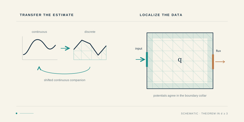
Can a continuous Carleman estimate tell us what a numerical boundary experiment can recover?

Our new paper connects these two questions.¹ It develops an elliptic transfer principle, then applies it to a discrete Calderón problem: determining an unknown potential from prescribed boundary values and the resulting boundary flux.

Give the discrete state a continuous companion

A piecewise-linear finite-element function generally belongs to \(H^1\), not \(H^2\). We cannot simply insert it into a continuous second-order Carleman estimate. The estimate also contains a large parameter \(s\), so ordinary convergence as the mesh size \(h\) tends to zero is not enough.

The construction shares its starting point with our parabolic transfer work. Given a discrete state, choose a shifted continuous equation whose Galerkin solution is exactly that state. Apply the continuous estimate to this more regular companion, and use weighted approximation estimates to transfer it back.

The resulting bound keeps the original discrete operator, without adding a stabilization term. For the radial weights used in continuation, the proof gives the sufficient range

This is a proved range, not an optimality claim. The paper verifies the numerical assumptions for conforming \(P_1\) finite elements with consistent or lumped mass on fitted, uniformly shape-regular meshes. Local refinement is allowed; quasi-uniformity is not required.

Put the input and the measurement in different places

Consider the discrete counterpart of

We prescribe Dirichlet values on one boundary patch, \(\Gamma_D\), and measure the variational flux on another, \(\Gamma_N\). The two patches can be chosen independently and may be disjoint.

The result has important prior assumptions. The dimension is \(d\ge3\), the domain and fitted meshes satisfy the paper's geometric conditions, and the bounded complex potentials agree in a fixed connected neighborhood of the entire boundary. Their discrete Dirichlet problems must also satisfy a mesh-uniform stability bound. Each accessible set contains a fixed nonempty patch in the interior of a boundary face.

Under these assumptions, boundary continuation first enlarges the observed flux region. Reciprocity exchanges input and observation; a second continuation enlarges the other side. This reduces the two-patch problem to a full-boundary comparison.

Keep the logarithm, and track the mesh error

Let \(\delta_{\mathrm{loc}}\) measure the difference between the two local boundary maps. For \(r>d/2\), the stability estimate is

Here \(\mathcal Q_h\) represents the potential as a function: the original coefficient for consistent mass, or control-volume constants for lumped mass, extended by zero outside the domain.

Localizing both input and observation preserves the single logarithm and the \(h^{1/2}\) remainder of the paper's full-data estimate. The continuation error is exponentially small in \(h^{-4/5}\); after entering the logarithm, it is absorbed by that mesh remainder.

The estimate separates measurement uncertainty from discretization. It does not assert exact recovery of an arbitrary potential at a fixed mesh. The useful conclusion is more specific: with the boundary agreement and stability assumptions in place, two small boundary patches retain the same stability scale as full-boundary data.